Score-Based Generative Modeling through Stochastic Differential Equations - notes

Posted at 2025-09-09 # ML/AI

デノイジング拡散モデル (DDPM) に来て, 拡散モデル (Sohl-Dickstein et al., 2015), および Langevin 動力学を用いたデノイジングスコアマッチング (DSMLD) は本質的に等価であることが示された. それらは離散有限ステップでの摂動を考え方の機軸としているが, 本論文においてはそれを連続無限に拡張するという, 確率微分方程式 (SDE) を用いた一般化をみる. 核となる考えは下図にまとめられている. idea

先行研究の整理

DSMLD (Song & Ermon, 2019)

— 記法と設計 —

データ分布: $p_{\text{data}}(\mathbf{x})$ .
摂動核: $p_σ\left(\tilde{\mathbf{x}}|\mathbf{x}\right)≔\mathcal{N}\left(\tilde{\mathbf{x}};\mathbf{x},σ^2\mathbf{I}\right)$ .
摂動後分布: $p_σ\left(\tilde{\mathbf{x}}\right)≔∫p_{\text{data}}(\mathbf{x})p_σ\left(\tilde{\mathbf{x}}|\mathbf{x}\right)\mathrm{d}\mathbf{x}$ .
正のノイズスケール列 $\left\lbrace σ_i\right\rbrace_{i=1}^N$ は狭義単調増加列, $\mathrm{i.e.}$ , $σ_{\text{min}}=σ_1<σ_2<\cdots<σ_N=σ_{\mathrm{max}}$ .
$σ_{\text{min}}$ は $p_{σ_{\text{min}}}(\mathbf{x})≈p_{\text{data}}(\mathbf{x})$ を満たすくらい十分に小さく, $σ_{\text{max}}$ は $p_{σ_{\text{max}}}(\mathbf{x})≈\mathcal{N}\left(\mathbf{x};\mathbf{0},σ_{\text{max}}\mathbf{I}\right)$ を満たすくらい十分に大きい.

— 訓練目標 —

DSM の重み付き和.

\mathbf{θ}^* = \mathop{\argmin}\limits_{\mathbf{θ}}\sum_{i=1}^Nσ_i^2\mathbb{E}_{p_{\text{data}}(\mathbf{x})}\mathbb{E}_{p_{σ_i}\left(\tilde{\mathbf{x}}|\mathbf{x}\right)}\left[\left\|\mathbf{s}_{\mathbf{θ}}\left(\tilde{\mathbf{x}},σ_i\right)-∇_{\mathbf{x}}\log p_{σ_i}\left(\tilde{\mathbf{x}}|\mathbf{x}\right)\right\|^2\right]

— サンプリング —

焼きなまし Langevin MCMC.

\begin{align} \mathbf{x}_i^m &≔ \mathbf{x}_i^{m-1}+ϵ_i\mathbf{s}_{\mathbf{θ}^*}\left(\mathbf{x}_i^{m-1},σ_i\right)+\sqrt{2ϵ_i}\mathbf{z}_i^m, m=1,2,\ldots,M \\ &\text{where }ϵ_i>0\text{ and }\mathbf{z}_i^m∼\mathcal{N}(\mathbf{0},\mathbf{I}) \end{align}

DDPM (Ho et al., 2020)

— 記法と設計 —

拡散スケジュール $\left\lbrace β_i\right\rbrace_{i=1}^N$ は, $0<β_1,β_2,\ldots,β_N<1$ を満たす.
拡散核: $\begin{align} &p\left(\mathbf{x}_i|\mathbf{x}_{i-1}\right)=\mathcal{N}\left(\mathbf{x}_i;\sqrt{1-β_i}\mathbf{x}_{i-1},β_i\mathbf{I}\right)\text{.} \\ ∴&p_{α_i}\left(\mathbf{x}_i|\mathbf{x}_0\right)=\mathcal{N}\left(\mathbf{x}_i;\sqrt{α_i}\mathbf{x}_{i-1},(1-α_i)\mathbf{I}\right) \\ &\text{where }α_i≔∏_{j=1}^i\left(1-β_j\right) \end{align}$
摂動後分布: $p_{α_i}\left(\tilde{\mathbf{x}}\right)≔∫p_{\text{data}}(\mathbf{x})p_{α_i}\left(\tilde{\mathbf{x}}|\mathbf{x}\right)\mathrm{d}\mathbf{x}$ .
ノイズスケールは $\mathbf{x}_N∼\mathcal{N}(\mathbf{0},\mathbf{I})$ となるように事前に決定される.
逆拡散核: $p_{θ}\left(\mathbf{x}_{i-1}|\mathbf{x}_i\right)=\mathcal{N}\left(\mathbf{x}_{i-1};\frac{1}{\sqrt{1-β_i}}\left(\mathbf{x}_i+β_i\mathbf{s}_{\mathbf{θ}}\left(x_i,i\right)\right),β_i\mathbf{I}\right)$ .

— 訓練目標 —

ELBO.

\mathbf{θ}^* = \mathop{\argmin}\limits_{\mathbf{θ}}\sum_{i=1}^N\left(1-α_i\right)\mathbb{E}_{p_{\text{data}}(\mathbf{x})}\mathbb{E}_{p_{α_i}\left(\tilde{\mathbf{x}}|\mathbf{x}\right)}\left[\left\|\mathbf{s}_{\mathbf{θ}}\left(\tilde{\mathbf{x}},i\right)-∇_{\mathbf{x}}\log p_{α_i}\left(\tilde{\mathbf{x}}|\mathbf{x}\right)\right\|^2\right]

— サンプリング —

Ancestral sampling.

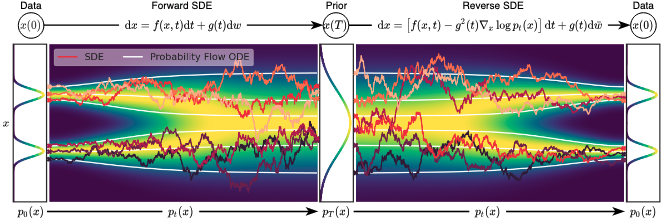
\begin{align} \mathbf{x}_{i-1} &= \frac{1}{\sqrt{1-β_i}}\left(\mathbf{x}_i+β_i\mathbf{s}_{\mathbf{θ}^*}\left(\mathbf{x}_i,i\right)\right)+\sqrt{β_i}\mathbf{z}_i\text{ , }i=N,N-1,\ldots,1 \\ &\text{where }\mathbf{z}_i∼\mathcal{N}(\mathbf{0},\mathbf{I}) \end{align}

SDE を用いたスコアベースモデル

下図がこの枠組みの概念図である. framework

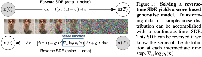
SDE による拡散過程のモデル化

境界条件 $\mathbf{x}(0)∼p_0$ (データ分布), および $\mathbf{x}(T)∼p_T$ (事前分布) を満たす, 連続時間 $t\in[0,T]$ を変数とする拡散過程 $\left\lbrace \mathbf{x}(t)\right\rbrace_{t=0}^T$ は次のような It $\text{\^{o}}$ (伊藤) SDE に対する解としてモデル化できる.

\mathrm{d}\mathbf{x} = \mathbf{f}(\mathbf{x},t)\mathrm{d}t+g(t)\mathrm{d}\mathbf{w}

ここで, $\mathbf{w}$ は標準 Wiener 過程 (a.k.a., Brown 運動), $\mathbf{f}(⋅,t):\mathbb{R}^d→\mathbb{R}^d$ は $\mathbf{x}(t)$ のドリフト係数とよばれるベクトル値関数, $g(⋅):\mathbb{R}→\mathbb{R}$ は $\mathbf{x}(t)$ の拡散係数とよばれるスカラー関数である. これらの係数が, $\mathbf{x}$ および $t$ に対し大域的 Lipschitz 条件を満たす限り, It $\text{\^{o}}$ SDE は一意な強解を持つ (Øksendal, 2003).

SDE による逆拡散過程のモデル化

逆拡散過程もまた $T$ から $0$ へと時間を遡る方向の拡散過程となり, 次の逆時間 SDE でモデル化される (Anderson, 1982).

\mathrm{d}\mathbf{x} = \left[\mathbf{f}(\mathbf{x},t)-g(t)^2∇_\mathbf{x}\log p_t(\mathbf{x})\right]\mathrm{d}t+g(t)\mathrm{d}\bar{\mathbf{w}}

ここで, $\bar{\mathbf{w}}$ は標準 Wiener 過程, $\mathrm{d}t$ は逆向き時間の無限小.

確率フロー ODE

定理. 拡散 / 逆拡散 SDE と同じ周辺確率密度 $\left\lbrace p_t(\mathbf{x})\right\rbrace_{t=0}^T$ を軌跡に持つ決定論的 ODE が存在し, それは以下で与えられる. この ODE を確率フロー ODE とよぶ.

\mathrm{d}\mathbf{x} = \left[\mathbf{f}(\mathbf{x},t)-\frac{1}{2}g(t)^2∇_{\mathbf{x}}\log p_t(\mathbf{x})\right]\mathrm{d}t

証明. 次の最も一般の形式を持つ SDE に対して証明する.

\mathrm{d}\mathbf{x} = \mathbf{f}(\mathbf{x},t)\mathrm{d}t+\mathbf{G}(\mathbf{x},t)\mathrm{d}\mathbf{w}

ここで, $\mathbf{f}(⋅,t):\mathbb{R}^d→\mathbb{R}^d$ はドリフト係数, $\mathbf{G}(⋅,t):\mathbb{R}^d→\mathbb{R}^{d×d}$ は拡散係数.

周辺分布 $p_t(\mathbf{x})$ の時間発展は次の Kolmogorov 前進 (a.k.a., Fokker-Planck) 方程式で与えられる.

\begin{align} &\space\space\space\space\frac{∂p_t(\mathbf{x})}{∂t} \\ &= -\sum_{i=1}^d\frac{∂}{∂x_i}\left[f_i(\mathbf{x},t)p_t(\mathbf{x})\right]+\frac{1}{2}\sum_{i=1}^d\sum_{j=1}^d\frac{∂^2}{∂x_i∂x_j}\left[\sum_{k=1}^dG_{ik}(\mathbf{x},t)G_{jk}(\mathbf{x},t)p_t(\mathbf{x})\right] \\ &= -\sum_{i=1}^d\frac{∂}{∂x_i}\left[f_i(\mathbf{x},t)p_t(\mathbf{x})\right] \\ &\space\space+\frac{1}{2}\sum_{i=1}^d\frac{∂}{∂x_i}\left[\sum_{j=1}^d\left\lbrace\frac{∂}{∂x_j}\left[\sum_{k=1}^dG_{ik}(\mathbf{x},t)G_{jk}(\mathbf{x},t)\right]p_t(\mathbf{x})+\sum_{k=1}^dG_{ik}(\mathbf{x},t)G_{jk}(\mathbf{x},t)p_t(\mathbf{x})\frac{∂}{∂x_j}\log p_t(\mathbf{x})\right\rbrace\right] \\ &= -\sum_{i=1}^d\frac{∂}{∂x_i}\left[f_i(\mathbf{x},t)p_t(\mathbf{x})\right] \\ &\space\space+\frac{1}{2}\sum_{i=1}^d\frac{∂}{∂x_i}\left[∇⋅\left[\mathbf{G}(\mathbf{x},t)\mathbf{G}(\mathbf{x},t)^{\mathrm{T}}\right]p_t(\mathbf{x})+\mathbf{G}(\mathbf{x},t)\mathbf{G}(\mathbf{x},t)^{\mathrm{T}}p_t(\mathbf{x})∇_{\mathbf{x}}\log p_t(\mathbf{x})\right] \\ &=-\sum_{i=1}^d\frac{∂}{∂x_i}\left[\left\lbrace f_i(\mathbf{x},t)-\frac{1}{2}\left[∇⋅\left[\mathbf{G}(\mathbf{x},t)\mathbf{G}(\mathbf{x},t)^{\mathrm{T}}\right]+\mathbf{G}(\mathbf{x},t)\mathbf{G}(\mathbf{x},t)^{\mathrm{T}}∇_{\mathbf{x}}\log p_t(\mathbf{x})\right]\right\rbrace p_t(\mathbf{x})\right] \\ &≔-\sum_{i=1}^d\frac{∂}{∂x_i}\left[\tilde{\mathbf{f}}_i(\mathbf{x},t)p_t(\mathbf{x})\right] \end{align}

結局これは, $\mathrm{d}\mathbf{x}=\tilde{\mathbf{f}}(\mathbf{x},t)\mathrm{d}t+\tilde{\mathbf{G}}(\mathbf{x},t)\mathrm{d}\mathbf{w}$ という SDE において, $\tilde{\mathbf{G}}(\mathbf{x},t)=\mathbf{O}$ とした ODE $\mathrm{d}\mathbf{x}=\tilde{\mathbf{f}}(\mathbf{x},t)\mathrm{d}t$ の Kolmogorov 前進方程式となっている. $\tilde{\mathbf{f}}(\mathbf{x},t)$ において, $\mathbf{G}(\mathbf{x},t)=g(t)\mathbf{I}$ とした特別の場合が確率フロー ODE である. $\square$

訓練目標

\mathbf{θ}^* = \mathop{\argmin}\limits_{\mathbf{θ}}\mathbb{E}_t\left\lbrace λ(t)\mathbb{E}_{\mathbf{x}(0)∼p_{\text{data}}(\mathbf{x})}\mathbb{E}_{\mathbf{x}(t)∼p_{0t}\left(\mathbf{x}(t)|\mathbf{x}(0)\right)}\left[\left\|\mathbf{s}_{\mathbf{θ}}\left(\mathbf{x}(t),t\right)-∇_{\mathbf{x}(t)}\log p_{0t}\left(\mathbf{x}(t)|\mathbf{x}(0)\right)\right\|^2\right]\right\rbrace

ここで, $λ:[0,T]→\mathbb{R}_{>0}$ は重み付け関数, $t∼U(0,T)$ . 評価のためには遷移核 $p_{0t}\left(\mathbf{x}(t)|\mathbf{x}(0)\right)$ を求める必要があるが, $\mathbf{f}(⋅,t)$ が Affine 変換ならそれは常に Gauss 分布となり閉形式でかける (Särkkä & Solin, 2019). しかし一般の場合には, Kolmogorov 前進方程式を解かなければならない.

サンプリング

逆拡散サンプラー

逆拡散 SDE の離散化.

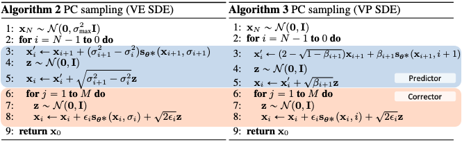
\begin{align} \mathbf{x}_i &= \mathbf{x}_{i+1}-\mathbf{f}_{i+1}\left(\mathbf{x}_{i+1}\right)+g_{i+1}^2\mathbf{s}_{θ^*}\left(\mathbf{x}_{i+1},i+1\right)+g_{i+1}\mathbf{z}_{i+1}\text{ , }i=N-1,N-2,\ldots,0 \\ &\text{where }\mathbf{z}_{i+1}∼\mathcal{N}(\mathbf{0},\mathbf{I}) \end{align}

予測器 - 修正器 (PC) サンプラー

逆拡散サンプラー (predictor) + 焼きなまし Langevin MCMC (corrector). PC sampling

確率フローサンプラー

確率フロー ODE の離散化.

\mathbf{x}_i = \mathbf{x}_{i+1}-\mathbf{f}_{i+1}\left(\mathbf{x}_{i+1}\right)-\frac{1}{2}g_{i+1}^2\mathbf{s}_{θ^*}\left(\mathbf{x}_{i+1},i+1\right)\text{ , }i=N-1,N-2,\ldots,0

これは決定論的ゆえサンプルを早く生成することが可能だが, 結局サンプル品質向上 (離散化誤差軽減) のためには多少のノイズを加えるのがよいとされている.

例: VE, VP SDE, およびその先へ

以上の議論を DSMLD と DDPM に適用する. 得られた 2 つの異なる SDE は, 分散の時間発展性に応じてそれぞれ分散爆発型 (VE) SDE, 分散保存型 (VP) SDE とよばれる.

VE SDE

DSMLD の各摂動核 $p_{σ_i}\left(\mathbf{x}_i|\mathbf{x}_{i-1}\right)$ に対応する $\mathbf{x}_i$ の分布は, 次の離散 Markov 鎖で与えられる.

\begin{align} \mathbf{x}_i &= \mathbf{x}_{i-1}+\sqrt{σ_i^2-σ_{i-1}^2}\mathbf{z}_{i-1}\text{ , }i=1,2,\ldots,N \\ &\text{where }\mathbf{z}_{i-1}∼\mathcal{N}(\mathbf{0},\mathbf{I}) \end{align}

$Δt=\frac{1}{N}$ , $t=\left\lbrace 0,\frac{1}{N},\cdots,\frac{N-1}{N}\right\rbrace$ とし, $N→∞$ の極限において 1 次近似までをとれば, 連続確率過程 $\mathbf{x}(t)$ として次の SDE を得る.

\mathrm{d}\mathbf{x} = \sqrt{\frac{\mathrm{d}σ^2(t)}{\mathrm{d}t}}\mathrm{d}\mathbf{w}

そして, 遷移核として次を得る.

p_{0t}\left(\mathbf{x}(t)|\mathbf{x}(0)\right) = \mathcal{N}\left(\mathbf{x}(t);\mathbf{x}(0),\left[σ^2(t)-σ^2(0)\right]\mathbf{I}\right)

また, 逆拡散サンプラー, および確率フローサンプラーとして以下を得る.

逆拡散サンプラー $\begin{align} \mathbf{x}_i &= \mathbf{x}_{i+1}+\left(σ_{i+1}^2-σ_i^2\right)\mathbf{s}_{\mathbf{θ}^*}\left(\mathbf{x}_{i+1},σ_{i+1}\right)+\sqrt{σ_{i+1}^2-σ_i^2}\mathbf{z}_{i+1}\text{ , }i=N-1,N-2,\ldots,0 \\ &\text{where }\mathbf{z}_{i+1}∼\mathcal{N}(\mathbf{0},\mathbf{I}) \end{align}$
確率フローサンプラー $\mathbf{x}_i = \mathbf{x}_{i+1}-\frac{1}{2}\left(σ_{i+1}^2-σ_i^2\right)\mathbf{s}_{\mathbf{θ}^*}\left(\mathbf{x}_{i+1},σ_{i+1}\right)\text{ , }i=N-1,N-2,\ldots,0$

VP SDE

DDPM の各摂動核 $p_{σ_i}\left(\mathbf{x}_i|\mathbf{x}_{i-1}\right)$ に対応する $\mathbf{x}_i$ の分布は, 次の離散 Markov 鎖で与えられる.

\begin{align} \mathbf{x}_i &= \sqrt{1-β_i}\mathbf{x}_{i-1}+\sqrt{β_i}\mathbf{z}_{i-1}\text{ , }i=1,2,\ldots,N \\ &\text{where }\mathbf{z}_{i-1}∼\mathcal{N}(\mathbf{0},\mathbf{I}) \end{align}

\mathrm{d}\mathbf{x} = -\frac{1}{2}β(t)\mathbf{x}\mathrm{d}t+\sqrt{β(t)}\mathrm{d}\mathbf{w}