supercalifragilisticexpialidocious

Koji Higasa Blog

Deep Unsupervised Learning using Nonequilibrium Thermodynamics - notes

Posted at # ML/AI

拡散モデルの原型となる論文. 表題の通り, 非平衡熱力学を下敷きにしており, 情報科学への応用, および定式化, 最終的な実装までをもやってのける強力な知性に驚嘆する. 美しいことにモデルの枠組みも非常に簡明で, 以下 2 つの双対的な過程より構成されている.

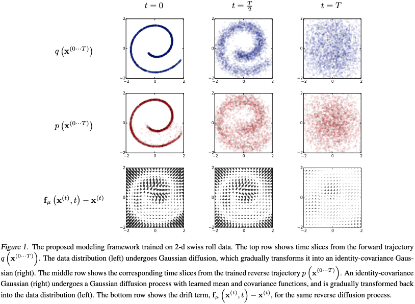
  1. 拡散過程: 所与の複雑なデータ分布から Gauss 分布や Laplace 分布などの単純な分布への変換, Fig. 1 でいえば, 青 (t=0t=0) から 青 (t=Tt=T) への変換.
  2. 逆拡散過程: 単純な分布から所与のデータ分布を再現しようとする変換, すなわち生成過程, Fig. 1 でいえば, 赤 (t=Tt=T) から 赤 (t=0t=0) への変換. framework

拡散過程の軌跡

拡散過程は, “データ分布 q(x(0))q(\mathbf{x}^{(0)}) が, 単純な分布 π(y)\pi(\mathbf{y}) に対する Markov 拡散核 Tπ(yy;β)T_{\pi}(\mathbf{y}|\mathbf{y}';β) (ここで ββ は拡散率) を繰り返し適用されることで, 段々と π(y)\pi(\mathbf{y}) に変換されていく過程” として, 次のように定式化される. ただし, 核のパラメータは多層パーセプトロンにより調整される.

π(y)=Tπ(yy;β)π(y)dy\pi(\mathbf{y}) = ∫T_{\pi}(\mathbf{y}|\mathbf{y}';β)\pi(\mathbf{y}')\mathrm{d}\mathbf{y}'

またその軌跡は, 拡散を TT ステップ行うとすれば, 次のような Markov 連鎖として与えられる.

q(x(0T))=q(x(0))t=1Tq(x(t)x(t1))q(x(t)x(t1))=Tπ(x(t)x(t1);βt)\begin{align} q\left(\mathbf{x}^{(0\cdots T)}\right) &= q\left(\mathbf{x}^{(0)}\right)∏_{t=1}^Tq\left(\mathbf{x}^{(t)}|\mathbf{x}^{(t-1)}\right) \\ q\left(\mathbf{x}^{(t)}|\mathbf{x}^{(t-1)}\right) &= T_{\pi}\left(\mathbf{x}^{(t)}|\mathbf{x}^{(t-1)};β_t\right) \end{align}

逆拡散過程の軌跡

拡散過程の定式化を振り返れば, 逆拡散過程の軌跡が p(x(T))=π(x(T))p\left(\mathbf{x}^{(T)}\right)=\pi\left(\mathbf{x}^{(T)}\right) として, 次のように与えられることは自明といってよい.

p(x(0T))=p(x(T))t=1Tp(x(t1)x(t))p\left(\mathbf{x}^{(0\cdots T)}\right) = p\left(\mathbf{x}^{(T)}\right)∏_{t=1}^Tp\left(\mathbf{x}^{(t-1)}|\mathbf{x}^{(t)}\right)

生成分布

逆拡散過程を通じて最終的に得られる生成分布は以下で与えられる.

    p(x(0))=p(x(0T))dx(1T)  ()=q(x(1T)x(0))q(x(1T)x(0))p(x(0T))dx(1T)=p(x(0T))q(x(1T)x(0))q(x(1T)x(0))dx(1T)=p(x(T))t=1Tp(x(t1)x(t))q(x(t)x(t1))q(x(1T)x(0))dx(1T)  ()=Eq(x(1T)x(0))[p(x(T))t=1Tp(x(t1)x(t))q(x(t)x(t1))]β0Eq(x(1T)x(0))[p(x(T))]  p(x(t1)x(t))q(x(t)x(t1))1\begin{align} &\space\space\space\space p\left(\mathbf{x}^{(0)}\right) \\ &= ∫p\left(\mathbf{x}^{(0\cdots T)}\right)\mathrm{d}\mathbf{x}^{(1\cdots T)}\space\space(*) \\ &= ∫\frac{q\left(\mathbf{x}^{(1\cdots T)}|\mathbf{x}^{(0)}\right)}{q\left(\mathbf{x}^{(1\cdots T)}|\mathbf{x}^{(0)}\right)}p\left(\mathbf{x}^{(0\cdots T)}\right)\mathrm{d}\mathbf{x}^{(1\cdots T)} \\ &= ∫\frac{p\left(\mathbf{x}^{(0\cdots T)}\right)}{q\left(\mathbf{x}^{(1\cdots T)}|\mathbf{x}^{(0)}\right)}q\left(\mathbf{x}^{(1\cdots T)}|\mathbf{x}^{(0)}\right)\mathrm{d}\mathbf{x}^{(1\cdots T)} \\ &= ∫p\left(\mathbf{x}^{(T)}\right)∏_{t=1}^T\frac{p\left(\mathbf{x}^{(t-1)}|\mathbf{x}^{(t)}\right)}{q\left(\mathbf{x}^{(t)}|\mathbf{x}^{(t-1)}\right)}q\left(\mathbf{x}^{(1\cdots T)}|\mathbf{x}^{(0)}\right)\mathrm{d}\mathbf{x}^{(1\cdots T)}\space\space(**) \\ &= \mathbb{E}_{q\left(\mathbf{x}^{(1\cdots T)}|\mathbf{x}^{(0)}\right)}\left[p\left(\mathbf{x}^{(T)}\right)∏_{t=1}^T\frac{p\left(\mathbf{x}^{(t-1)}|\mathbf{x}^{(t)}\right)}{q\left(\mathbf{x}^{(t)}|\mathbf{x}^{(t-1)}\right)}\right] \\ &\mathop{→}\limits_{β→0} \mathbb{E}_{q\left(\mathbf{x}^{(1\cdots T)}|\mathbf{x}^{(0)}\right)}\left[p\left(\mathbf{x}^{(T)}\right)\right]\space\space∵\frac{p\left(\mathbf{x}^{(t-1)}|\mathbf{x}^{(t)}\right)}{q\left(\mathbf{x}^{(t)}|\mathbf{x}^{(t-1)}\right)}→1 \end{align}

近似のない式変形を行ったが, 各段階でそれぞれの式の表す意味は大きく異なる. ()(*) においては, p(x(0T))p\left(\mathbf{x}^{(0\cdots T)}\right) の規格化定数が計算不能ゆえ, 積分も計算不能であった. しかし ()(**) において, 焼きなまし重点サンプリング (AIS), ないしは物理的な視点から Jarzynski 等式の発想により, 規格化定数は拡散過程と逆拡散過程の比として現れるようになった. そして最終的に, 拡散率を 00 とする極限, すなわち統計力学的な見方では準静的過程とよばれる過程を考えることで, その比すらも消失した. ここにおいてはもはや積分計算の際に, Monte Carlo 法による多数サンプリングを必要とせず, q(x(1T)x(0))q\left(\mathbf{x}^{(1\cdots T)}|\mathbf{x}^{(0)}\right) から単一サンプリングするだけで結果を導けるようになった.

訓練

訓練とは, 次で与えられる対数尤度 LL を最大化することである. しかし実際の問題は, その下限 KK を最大化する逆拡散過程を見つけることである, i.e.\mathrm{i.e.}, p^(x(t1)x(t))arg maxp(x(t1)x(t))K\hat{p}\left(\mathbf{x}^{(t-1)}|\mathbf{x}^{(t)}\right)≔\mathop{\argmax}\limits_{p\left(\mathbf{x}^{(t-1)}|\mathbf{x}^{(t)}\right)}K.

    LEq(x(0))[logp(x(0))]=q(x(0))logp(x(0))dx(0)=q(x(0))log[Eq(x(1T)x(0))[p(x(T))t=1Tp(x(t1)x(t))q(x(t)x(t1))]]dx(0)q(x(0))Eq(x(1T)x(0))[log[p(x(T))t=1Tp(x(t1)x(t))q(x(t)x(t1))]]dx(0)     Jensen の定理 (準静的過程で等号成立)=q(x(0T))log[p(x(T))t=1Tp(x(t1)x(t))q(x(t)x(t1))]dx(0T)K\begin{align} &\space\space\space\space L \\ &≔ \mathbb{E}_{q\left(\mathbf{x}^{(0)}\right)}\left[\log p\left(\mathbf{x}^{(0)}\right)\right] \\ &= ∫q\left(\mathbf{x}^{(0)}\right)\log p\left(\mathbf{x}^{(0)}\right)\mathrm{d}\mathbf{x}^{(0)} \\ &= ∫q\left(\mathbf{x}^{(0)}\right)\log\left[\mathbb{E}_{q\left(\mathbf{x}^{(1\cdots T)}|\mathbf{x}^{(0)}\right)}\left[p\left(\mathbf{x}^{(T)}\right)∏_{t=1}^T\frac{p\left(\mathbf{x}^{(t-1)}|\mathbf{x}^{(t)}\right)}{q\left(\mathbf{x}^{(t)}|\mathbf{x}^{(t-1)}\right)}\right]\right]\mathrm{d}\mathbf{x}^{(0)} \\ &≥ ∫q\left(\mathbf{x}^{(0)}\right)\mathbb{E}_{q\left(\mathbf{x}^{(1\cdots T)}|\mathbf{x}^{(0)}\right)}\left[\log\left[p\left(\mathbf{x}^{(T)}\right)∏_{t=1}^T\frac{p\left(\mathbf{x}^{(t-1)}|\mathbf{x}^{(t)}\right)}{q\left(\mathbf{x}^{(t)}|\mathbf{x}^{(t-1)}\right)}\right]\right]\mathrm{d}\mathbf{x}^{(0)} \\ &\space\space\space\space∵\text{ Jensen の定理 (準静的過程で等号成立)} \\ &= ∫q\left(\mathbf{x}^{(0\cdots T)}\right)\log\left[p\left(\mathbf{x}^{(T)}\right)∏_{t=1}^T\frac{p\left(\mathbf{x}^{(t-1)}|\mathbf{x}^{(t)}\right)}{q\left(\mathbf{x}^{(t)}|\mathbf{x}^{(t-1)}\right)}\right]\mathrm{d}\mathbf{x}^{(0\cdots T)} \\ &≔ K \end{align}

K を解析的に計算可能な形へ書き換える

p(x(T))p\left(\mathbf{x}^{(T)}\right) のエントロピー Hp(x(T))H_p\left(\mathbf{x}^{(T)}\right) を導入 —

    K=q(x(0T))t=1Tlog[p(x(t1)x(t))q(x(t)x(t1))]dx(0T)  +q(x(0T))logp(x(T))dx(0T)=t=1Tq(x(0T))log[p(x(t1)x(t))q(x(t)x(t1))]dx(0T)  +q(x(T))logp(x(T))dx(T)=t=2Tq(x(0T))log[p(x(t1)x(t))q(x(t)x(t1))]dx(0T)  +q(x(0),x(1))log[p(x(0)x(1))q(x(1)x(0))]dx(0)dx(1)  Hp(x(T))\begin{align} &\space\space\space\space K \\ &= ∫q\left(\mathbf{x}^{(0\cdots T)}\right)\sum_{t=1}^T\log\left[\frac{p\left(\mathbf{x}^{(t-1)}|\mathbf{x}^{(t)}\right)}{q\left(\mathbf{x}^{(t)}|\mathbf{x}^{(t-1)}\right)}\right]\mathrm{d}\mathbf{x}^{(0\cdots T)} \\ &\space\space+∫q\left(\mathbf{x}^{(0\cdots T)}\right)\log p\left(\mathbf{x}^{(T)}\right)\mathrm{d}\mathbf{x}^{(0\cdots T)} \\ &= \sum_{t=1}^T∫q\left(\mathbf{x}^{(0\cdots T)}\right)\log\left[\frac{p\left(\mathbf{x}^{(t-1)}|\mathbf{x}^{(t)}\right)}{q\left(\mathbf{x}^{(t)}|\mathbf{x}^{(t-1)}\right)}\right]\mathrm{d}\mathbf{x}^{(0\cdots T)} \\ &\space\space+∫q\left(\mathbf{x}^{(T)}\right)\log p\left(\mathbf{x}^{(T)}\right)\mathrm{d}\mathbf{x}^{(T)} \\ &= \sum_{t=2}^T∫q\left(\mathbf{x}^{(0\cdots T)}\right)\log\left[\frac{p\left(\mathbf{x}^{(t-1)}|\mathbf{x}^{(t)}\right)}{q\left(\mathbf{x}^{(t)}|\mathbf{x}^{(t-1)}\right)}\right]\mathrm{d}\mathbf{x}^{(0\cdots T)} \\ &\space\space+∫q\left(\mathbf{x}^{(0)},\mathbf{x}^{(1)}\right)\log\left[\frac{p\left(\mathbf{x}^{(0)}|\mathbf{x}^{(1)}\right)}{q\left(\mathbf{x}^{(1)}|\mathbf{x}^{(0)}\right)}\right]\mathrm{d}\mathbf{x}^{(0)}\mathrm{d}\mathbf{x}^{(1)} \\ &\space\space-H_p\left(\mathbf{x}^{(T)}\right) \\ \end{align}

t=0t=0 におけるエッジ効果を除去 —

p(x(0)x(1))π(x(1))=q(x(1)x(0))π(x(0))p\left(\mathbf{x}^{(0)}|\mathbf{x}^{(1)}\right)\pi\left(\mathbf{x}^{(1)}\right)=q\left(\mathbf{x}^{(1)}|\mathbf{x}^{(0)}\right)\pi\left(\mathbf{x}^{(0)}\right) と考える.

    K=t=2Tq(x(0T))log[p(x(t1)x(t))q(x(t)x(t1))]dx(0T)  +q(x(0),x(1))log[q(x(1)x(0))π(x(0))q(x(1)x(0))π(x(1))]dx(0)dx(1)  Hp(x(T))=t=2Tq(x(0T))log[p(x(t1)x(t))q(x(t)x(t1))]dx(0T)  +q(x(0),x(1))log[π(x(0))π(x(1))]dx(0)dx(1)  Hp(x(T))=t=2Tq(x(0T))log[p(x(t1)x(t))q(x(t)x(t1))]dx(0T)  +Hq,π(x(0))Hq,π(x(1))  Hp(x(T))=t=2Tq(x(0T))log[p(x(t1)x(t))q(x(t)x(t1))]dx(0T)  Hp(x(T))\begin{align} &\space\space\space\space K \\ &= \sum_{t=2}^T∫q\left(\mathbf{x}^{(0\cdots T)}\right)\log\left[\frac{p\left(\mathbf{x}^{(t-1)}|\mathbf{x}^{(t)}\right)}{q\left(\mathbf{x}^{(t)}|\mathbf{x}^{(t-1)}\right)}\right]\mathrm{d}\mathbf{x}^{(0\cdots T)} \\ &\space\space+∫q\left(\mathbf{x}^{(0)},\mathbf{x}^{(1)}\right)\log\left[\frac{q\left(\mathbf{x}^{(1)}|\mathbf{x}^{(0)}\right)\pi\left(\mathbf{x}^{(0)}\right)}{q\left(\mathbf{x}^{(1)}|\mathbf{x}^{(0)}\right)\pi\left(\mathbf{x}^{(1)}\right)}\right]\mathrm{d}\mathbf{x}^{(0)}\mathrm{d}\mathbf{x}^{(1)} \\ &\space\space-H_p\left(\mathbf{x}^{(T)}\right) \\ &= \sum_{t=2}^T∫q\left(\mathbf{x}^{(0\cdots T)}\right)\log\left[\frac{p\left(\mathbf{x}^{(t-1)}|\mathbf{x}^{(t)}\right)}{q\left(\mathbf{x}^{(t)}|\mathbf{x}^{(t-1)}\right)}\right]\mathrm{d}\mathbf{x}^{(0\cdots T)} \\ &\space\space+∫q\left(\mathbf{x}^{(0)},\mathbf{x}^{(1)}\right)\log\left[\frac{\pi\left(\mathbf{x}^{(0)}\right)}{\pi\left(\mathbf{x}^{(1)}\right)}\right]\mathrm{d}\mathbf{x}^{(0)}\mathrm{d}\mathbf{x}^{(1)} \\ &\space\space-H_p\left(\mathbf{x}^{(T)}\right) \\ &= \sum_{t=2}^T∫q\left(\mathbf{x}^{(0\cdots T)}\right)\log\left[\frac{p\left(\mathbf{x}^{(t-1)}|\mathbf{x}^{(t)}\right)}{q\left(\mathbf{x}^{(t)}|\mathbf{x}^{(t-1)}\right)}\right]\mathrm{d}\mathbf{x}^{(0\cdots T)} \\ &\space\space+H_{q,\pi}\left(\mathbf{x}^{(0)}\right)-H_{q,\pi}\left(\mathbf{x}^{(1)}\right) \\ &\space\space-H_p\left(\mathbf{x}^{(T)}\right) \\ &= \sum_{t=2}^T∫q\left(\mathbf{x}^{(0\cdots T)}\right)\log\left[\frac{p\left(\mathbf{x}^{(t-1)}|\mathbf{x}^{(t)}\right)}{q\left(\mathbf{x}^{(t)}|\mathbf{x}^{(t-1)}\right)}\right]\mathrm{d}\mathbf{x}^{(0\cdots T)} \\ &\space\space-H_p\left(\mathbf{x}^{(T)}\right) \\ \end{align}

最後の変形は拡散核を適切に設計していれば, π\pi に対する qq の交差エントロピーが tN,Hq,π(x(t))=Eq(x(t))[logπ(x(t))]=Const.∀t∈\mathbb{N}, H_{q,\pi}\left(\mathbf{x}^{(t)}\right)=-\mathbb{E}_{q\left(\mathbf{x}^{(t)}\right)}\left[\log\pi\left(\mathbf{x}^{(t)}\right)\right]=\mathrm{Const.} と考えられることによる.

— 事後分布 q(x(t1)x(0))q\left(\mathbf{x}^{(t-1)}|\mathbf{x}^{(0)}\right) に着目 —

拡散過程は Markov 過程なので, 条件に x(0)\mathbf{x}^{(0)} が入ったところで影響はなく以下が成り立つ.

t2,    q(x(t)x(t1))=q(x(t)x(t1),x(0))=q(x(t1)x(t),x(0))q(x(t)x(0))q(x(t1)x(0))   Bayes の定理\begin{align} ∀t≥2,&\space\space\space\space q\left(\mathbf{x}^{(t)}|\mathbf{x}^{(t-1)}\right) \\ &= q\left(\mathbf{x}^{(t)}|\mathbf{x}^{(t-1)},\mathbf{x}^{(0)}\right) \\ &= \frac{q\left(\mathbf{x}^{(t-1)}|\mathbf{x}^{(t)},\mathbf{x}^{(0)}\right)q\left(\mathbf{x}^{(t)}|\mathbf{x}^{(0)}\right)}{q\left(\mathbf{x}^{(t-1)}|\mathbf{x}^{(0)}\right)}\space\space∵\text{ Bayes の定理} \end{align}

したがって KK は次のように書き直せる.

    K=t=2Tq(x(0T))log[p(x(t1)x(t))q(x(t1)x(t),x(0))q(x(t1)x(0))q(x(t)x(0))]dx(0T)  Hp(x(T))=t=2Tq(x(0T))log[p(x(t1)x(t))q(x(t1)x(t),x(0))]dx(0T)  +t=2T[Hq(x(t)x(0))Hq(x(t1)x(0))]  Hp(x(T))=t=2Tq(x(0),x(t))DKL(q(x(t1)x(t),x(0))p(x(t1)x(t)))dx(0)dx(t)  +Hq(x(T)x(0))Hq(x(1)x(0))  Hp(x(T))\begin{align} &\space\space\space\space K \\ &= \sum_{t=2}^T∫q\left(\mathbf{x}^{(0\cdots T)}\right)\log\left[\frac{p\left(\mathbf{x}^{(t-1)}|\mathbf{x}^{(t)}\right)}{q\left(\mathbf{x}^{(t-1)}|\mathbf{x}^{(t)},\mathbf{x}^{(0)}\right)}\frac{q\left(\mathbf{x}^{(t-1)}|\mathbf{x}^{(0)}\right)}{q\left(\mathbf{x}^{(t)}|\mathbf{x}^{(0)}\right)}\right]\mathrm{d}\mathbf{x}^{(0\cdots T)} \\ &\space\space-H_p\left(\mathbf{x}^{(T)}\right) \\ &= \sum_{t=2}^T∫q\left(\mathbf{x}^{(0\cdots T)}\right)\log\left[\frac{p\left(\mathbf{x}^{(t-1)}|\mathbf{x}^{(t)}\right)}{q\left(\mathbf{x}^{(t-1)}|\mathbf{x}^{(t)},\mathbf{x}^{(0)}\right)}\right]\mathrm{d}\mathbf{x}^{(0\cdots T)} \\ &\space\space+\sum_{t=2}^T\left[H_q\left(\mathbf{x}^{(t)}|\mathbf{x}^{(0)}\right)-H_q\left(\mathbf{x}^{(t-1)}|\mathbf{x}^{(0)}\right)\right] \\ &\space\space-H_p\left(\mathbf{x}^{(T)}\right) \\ &= -\sum_{t=2}^T∫q\left(\mathbf{x}^{(0)},\mathbf{x}^{(t)}\right)D_{KL}\left(q\left(\mathbf{x}^{(t-1)}|\mathbf{x}^{(t)},\mathbf{x}^{(0)}\right)||p\left(\mathbf{x}^{(t-1)}|\mathbf{x}^{(t)}\right)\right)\mathrm{d}\mathbf{x}^{(0)}\mathrm{d}\mathbf{x}^{(t)} \\ &\space\space+H_q\left(\mathbf{x}^{(T)}|\mathbf{x}^{(0)}\right)-H_q\left(\mathbf{x}^{(1)}|\mathbf{x}^{(0)}\right) \\ &\space\space-H_p\left(\mathbf{x}^{(T)}\right) \\ \end{align}

第二の分布 r(x(t))r\left(\mathbf{x}^{(t)}\right) の導入

十分滑らかな r(x(t))r\left(\mathbf{x}^{(t)}\right) の導入により, 摂動として外部情報を取り込むことで, 理論の軽微な修正のみで事前分布 p(x(0))p\left(\mathbf{x}^{(0)}\right) の再現を超えた柔軟な生成タスクを可能にする. ただし, r(x(t))r\left(\mathbf{x}^{(t)}\right) の導入によっても閉形式となれば, 当然摂動近似によらず厳密計算が可能である.

修正逆拡散分布 p~(x(t))\tilde{p}\left(\mathbf{x}^{(t)}\right) を第二の分布を導入して次のようにかく.

p~(x(t))=1Z~tp(x(t))r(x(t))\tilde{p}\left(\mathbf{x}^{(t)}\right) = \frac{1}{\tilde{Z}_t}p\left(\mathbf{x}^{(t)}\right)r\left(\mathbf{x}^{(t)}\right)

さらに, 修正 Markov 逆拡散核 p~(x(t)x(t+1))\tilde{p}\left(\mathbf{x}^{(t)}|\mathbf{x}^{(t+1)}\right) を用いれば次のように書き直せる.

p~(x(t))=p~(x(t)x(t+1))p~(x(t+1))dx(t+1)p(x(t))r(x(t))Z~t=p~(x(t)x(t+1))p(x(t+1))r(x(t+1))Z~t+1dx(t+1)p(x(t))=p~(x(t)x(t+1))Z~tr(x(t+1))Z~t+1r(x(t))p(x(t+1))dx(t+1)\begin{align} &\tilde{p}\left(\mathbf{x}^{(t)}\right) = ∫\tilde{p}\left(\mathbf{x}^{(t)}|\mathbf{x}^{(t+1)}\right)\tilde{p}\left(\mathbf{x}^{(t+1)}\right)\mathrm{d}\mathbf{x}^{(t+1)} \\ ⇔ &\frac{p\left(\mathbf{x}^{(t)}\right)r\left(\mathbf{x}^{(t)}\right)}{\tilde{Z}_t} = ∫\tilde{p}\left(\mathbf{x}^{(t)}|\mathbf{x}^{(t+1)}\right)\frac{p\left(\mathbf{x}^{(t+1)}\right)r\left(\mathbf{x}^{(t+1)}\right)}{\tilde{Z}_{t+1}}\mathrm{d}\mathbf{x}^{(t+1)} \\ ⇔ &p\left(\mathbf{x}^{(t)}\right) = ∫\tilde{p}\left(\mathbf{x}^{(t)}|\mathbf{x}^{(t+1)}\right)\frac{\tilde{Z}_tr\left(\mathbf{x}^{(t+1)}\right)}{\tilde{Z}_{t+1}r\left(\mathbf{x}^{(t)}\right)}p\left(\mathbf{x}^{(t+1)}\right)\mathrm{d}\mathbf{x}^{(t+1)} \end{align}

したがって, 修正逆拡散過程は以下のようにかける.

p~(x(t)x(t+1))=p(x(t)x(t+1))Z~t+1r(x(t))Z~tr(x(t+1))1Z~t(x(t+1))p(x(t)x(t+1))r(x(t))\begin{align} \tilde{p}\left(\mathbf{x}^{(t)}|\mathbf{x}^{(t+1)}\right) &= p\left(\mathbf{x}^{(t)}|\mathbf{x}^{(t+1)}\right)\frac{\tilde{Z}_{t+1}r\left(\mathbf{x}^{(t)}\right)}{\tilde{Z}_tr\left(\mathbf{x}^{(t+1)}\right)} \\ &≔ \frac{1}{\tilde{Z}_t\left(\mathbf{x}^{(t+1)}\right)}p\left(\mathbf{x}^{(t)}|\mathbf{x}^{(t+1)}\right)r\left(\mathbf{x}^{(t)}\right) \end{align}

逆拡散過程のエントロピー Hq(x(t1)x(t))H_q\left(\mathbf{x}^{(t-1)}|\mathbf{x}^{(t)}\right)

Hq(x(t1)x(t))H_q\left(\mathbf{x}^{(t-1)}|\mathbf{x}^{(t)}\right) は解析的に計算可能な上界, および下界によって評価可能である. この評価は逆拡散過程の精度を測るうえで重要である. Bayes の定理により以下の不等式を得る.

Hq(x(t)x(t1))+Hq(x(t1)x(0))Hq(x(t)x(0))Hq(x(t1)x(t))Hq(x(t)x(t1))H_q\left(\mathbf{x}^{(t)}|\mathbf{x}^{(t-1)}\right)+H_q\left(\mathbf{x}^{(t-1)}|\mathbf{x}^{(0)}\right)-H_q\left(\mathbf{x}^{(t)}|\mathbf{x}^{(0)}\right)≤H_q\left(\mathbf{x}^{(t-1)}|\mathbf{x}^{(t)}\right)≤H_q\left(\mathbf{x}^{(t)}|\mathbf{x}^{(t-1)}\right)